Sorting and Searching
Sorting and Searching is one of the most vital topic in DSA. Storing and retrieving information is one of the most common application of computers now-a-days. According to time the amount of data and information stored and accessed via computer has turned to huge databases. So many techniques and algorithms have been developed to efficiently maintain and process information in databases. The processes of looking up a particular data record in the database is called searching. The process of ordering the records in a database is called Sorting. Sorting and searching together constitute a major area of study in computational methods. Both of them are very important field of study in data structure and algorithms. Let us discuss about both the topics in detail here.
What is searching?
Searching is the process of finding a particular item in a collection of items. A search typically answers whether the item is present in the collection or not. Searching requires a key field such as name, ID, code which is related to the target item. When the key field of a target item is found, a pointer to the target item is returned. The pointer may be an address, an index into a vector or array, or some other indication of where to find the target. If a matching key field isn’t found, the user is informed.
The most common searching algorithms are:
- Linear search
- Binary search
- Interpolation search
- Hash table
Linear Search Algorithm
Linear Search Algorithm is the simplest search algorithm. In this search algorithm a sequential search is made over all the items one by one to search for the targeted item. Each item is checked in sequence until the match is found. If the match is found, particular item is returned otherwise the search continues till the end.
Algorithm
LinearSearch ( Array A, Value x)

Step 1: Set i to 1

Step 2: if i > n then go to step 7

Step 3: if A[i] = x then go to step 6

Step 4: Set i to i + 1

Step 5: Go to Step 2

Step 6: Print Element x Found at index i and go to step 8

Step 7: Print element not found

Step 8: Exit
Linear Search Example
Let us take an example of an array A[7]={5,2,1,6,3,7,8}. Array A has 7 items. Let us assume we are looking for 7 in the array. Targeted item=7.
Here, we have
A[7]={5,2,1,6,3,7,8}
X=7
At first, When i=0 (A[0]=5; X=7) not matched
i++ now, i=1 (A[1]=2; X=7) not matched
i++ now, i=2(A[2])=1; X=7)not matched
…
….
i++ when, i=5(A[5]=7; X=7) Match Found
Hence, Element X=7 found at index 5.
Linear search is rarely used practically. The time complexity of above algorithm is O(n).
int linearSearch(int values[], int target, int n)
{
    for(int i = 0; i < n; i++)
    {
        if (values[i] == target)
        {
            return i;
        }
    }
    return -1;
}
Binary Search Algorithm
Binary Search Algorithm is fast according to run time complexity. This algorithm works on the basis of divide and conquer rule. In this algorithm we have to sort the data collection in ascending order first then search for the targeted item by comparing the middle most item of the collection. If match found, the index of item is returned. If the middle item is greater than the targeted item, the item is searched in the sub-array to the left of the middle item. Otherwise, the item is searched for in the sub-array to the right of the middle item. This process continues on the sub-array as well until the size of the sub array reduces to zero.
Algorithm
Step 1: Data list must be ordered list in ascending order.

Step 2: Probe middle of list

Step 3: If target equals list[mid], FOUND.

Step 4: If target < list[mid], discard 1/2 of list between list[mid] and list[last].

Step 5: If target > list[mid], discard 1/2 of list between list[first] and list[mid].

Step 6: Continue searching the shortened list until either the target is found, or there are no elements to probe.
Binary Search Example
Let us take an example of an array A[16]={1,2,3,4,6,7,8,10,12,13,15,16,18,19,20,22}. The array is sorted and contains 16 items. We are looking for item 19 in this list.
Here, we have
A[16]={1,2,3,4,6,7,8,10,12,13,15,16,18,19,20,22}
X=19
Let us first divide it into two smaller arrays of 8 items each. The first 8 items in a sub array and another 8 in another sub array. A1={1,2,3,4,6,7,8,10} and A2={12,13,15,16,18,19,20,22}
As 10 and 12 are the middle items of this ordered array, we know 19 is greater than the middle numbers that means we don’t require to look for the targeted item in first sub array. Let us search in the second subarray A2={12,13,15,16,18,19,20,22}
In the second array we have 8 items. Let’s divide them into two equal arrays and check the middle items. Here the middle items are 16 and 18. As 19 is greater than both of them, we don’t need to look in the first four items of this subarray. A21={12,13,15,15} and A22={18,19,20,22}
Let us look in the last four items sub array A22={18,19,20,22}. Let us again divide it to subarrays A221={18,19) and A222={20,22}. Here the middle items are 19 and 20. Hence, we found the target item 19 in first subarray.
Time complexity of Binary search algorithm is O(logn) or O(n).
int binarySearch(int values[], int len, int target)
{
    int max = (len - 1);
    int min = 0;
    int guess; // index of middle elements
    int step = 0; // to find out in how many steps we completed the search
    while(max >= min)
    {
        guess = (max + min) / 2;
        // we made the first guess, incrementing step by 1
        step++;
        if(values[guess] == target)
        {
            printf("Number of steps required for search: %d \n", step);
            return guess;
        }
        else if(values[guess] > target)
        {
        // target would be in the left half
        max = (guess - 1);
        }
        else
        {
        // target would be in the right half
        min = (guess + 1);
        }
    }
    // Element not found
    return -1;
}
Interpolation Search Algorithm
Interpolation Search Algorithm is an improvement of Binary Search. It works on the probing position of the required item. It works properly in sorted and equally distributed data lists.
Algorithm
Step 1: Start searching data from middle of the list.

Step 2: If it is a match, return the index of the item, and exit.

Step 3: If it is not a match, probe position.

Step 4: Divide the list using probing formula and find the new middle.

Step 5: If data is greater than middle, search in higher sub-list.

Step 6: If data is smaller than middle, search in lower sub-list.

Step 7: Repeat until match.
To divide the list into two sub lists, we use mid = Lo + ((Hi – Lo) / (A[Hi] – A[Lo])) * (X – A[Lo])
Where,
A = list
Lo = Lowest index of the list
Hi = Highest index of the list
A[n] = Value stored at index n in the list
Runtime complexity of interpolation search algorithm is Ο(log (log n)).
Hash Table
Hash table is a data structure that stores data in array format. Here each data has its own unique index. If you know the index value of required data, searching is very easy and fast. Hash Table uses an array as a storage medium and uses hash technique to generate an index where an element is to be inserted or is to be located from. Insert, Delete and Search are primary basic operations that we can perform easily and quickly in a hash table. It works on key, value pair.
What is sorting?
Sorting is the process of placing elements from a collection in some kind of order. For example, a list of words could be sorted alphabetically or by length. Efficient sorting is important to optimize the use of other algorithms that require sorted lists to work correctly.
Importance of sorting
- To represent data in more readable format.
- Optimize data searching to high level.
The most common sorting algorithms are:
- Bubble Sort
- Insertion Sort
- Selection Sort
- Quick Sort
- Merge Sort
- Shell Sort
Bubble Sort
Bubble sort is the simplest sorting algorithm. It is based on comparison where each adjacent pair of element is compared and swapped if they are not in order. It works by repeatedly stepping through the list to be sorted, comparing two items at a time and swapping them if they are in the wrong order. The pass through the list is repeated until no swaps are needed, which means the list is sorted. This algorithm is not suitable for huge data sets. Average and worst case time complexity of this algorithm are of Ο(n2) where n is the number of items.
Algorithm
for i=N-1 to 2 {

set swap flag to false

for j=1 to i {

if list[j-1] > list[j]

swap list[j-1] and list[j]

set swap flag to true

}

if swap flag is false, break. The list is sorted.

}
[NOTE: In each pass, the largest item “bubbles” down the list until it settles in its final position. This is where bubble sort gets its name.]
Example,
Suppose we have a list of array of 5 elements A[5]={40,50,30,20,10}. We have to sort this array using bubble sort algorithm.

We observe in algorithm that Bubble Sort compares each pair of array element unless the whole array is completely sorted in an ascending order. After every iteration the highest values settles down at the end of the array. Hence, the next iteration need not include already sorted elements.
void bubbleSort(int arr[], int n)
{
    int i, j, temp;
    for(i = 0; i < n; i++)
    {
        for(j = 0; j < n-i-1; j++)
        {
            if( arr[j] > arr[j+1])
            {
// swap the elements
                temp = arr[j];
                arr[j] = arr[j+1];
                arr[j+1] = temp;
            }
        }
}
Selection Sort
Selection sort is an in-place comparison sort algorithm. In this algorithm, we repeatedly select the smallest remaining element and move it to the end of a growing sorted list. It is one of the simplest sorting algorithm. Selection sort is known for its simplicity. It has performance advantages over more complicated algorithms in certain situations.
This algorithm is not suitable for large data sets as its average and worst case complexities are of Ο(n2), where n is the number of items.
Algorithm
Step 1: Set MIN to location 0

Step 2: Search the minimum element in the list

Step 3: Swap with value at location MIN

Step 4: Increment MIN to point to next element

Step 5: Repeat until list is sorted
Example,
Let us assume an array A[10]={45,20,40,05,15,25,50,35,30,10}. We have to sort this array using selection sort.

In this algorithm we have to find the minimum value in the list first. Then, Swap it with the value in the first position. After that, Start from the second position and repeat the steps above for remainder of the list.
// function to look for smallest element in the given subarray
int indexOfMinimum(int arr[], int startIndex, int n)
{
    int minValue = arr[startIndex];
    int minIndex = startIndex;
    for(int i = minIndex + 1; i < n; i++)
    {
        if(arr[i] < minValue)
        {
            minIndex = i;
            minValue = arr[i];
        }
    }
    return minIndex;
}

void selectionSort(int arr[], int n)
{
    for(int i = 0; i < n; i++)
    {
        int index = indexOfMinimum(arr, i, n);
        swap(arr, i, index);
    }
}
Insertion Sort
Insertion sort is an in-place sorting algorithm based on comparison. It is a simple algorithm where a sorted sub list is maintained by entering on element at a time. An element which is to be inserted in this sorted sub-list has to find its appropriate location and then it has to be inserted there. That is the reason why it is named so. This algorithm is not suitable for large data set.
Average and worst case time complexity of the algorithm is Ο(n2), where n is the number of items.
Algorithm
Step 1: If it is the first element, it is already sorted. return 1;

Step 2: Pick next element

Step 3: Compare with all elements in the sorted sub-list

Step 4: Shift all the elements in the sorted sub-list that is greater than the value to be sorted

Step 5: Insert the value

Step 6: Repeat until list is sorted
Example,
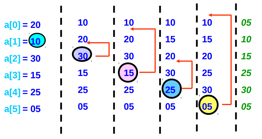
Let us take an example of an array A[6]={20,10,30,15,25,05}. We have to sort this array using insertion sort.

void insertionSort(int arr[], int length)
{
    int i, j, key;
    for (i = 1; i < length; i++)
    {
        j = i;
        while (j > 0 && arr[j - 1] > arr[j])
        {
            key = arr[j];
            arr[j] = arr[j - 1];
            arr[j - 1] = key;
            j--;
        }
    }
}
Quick Sort
Quick sort is a well-known sorting algorithm. It is highly efficient and also known as partition exchange sort. In this sorting algorithm the array is divided into 2 sub array. One contain smaller values than pivot value and other array contain elements having greater values than pivot value. Pivot is an element that is used to compare and divide the elements of the main array into two. Quick sort partitions an array and then calls itself recursively twice to sort the two resulting sub arrays. This algorithm is quite efficient for large data sets.
The Average and worst case complexity are of this algorithm is Ο(n2), where n is the number of items.
Algorithm
Step 1: Choose the highest index value has pivot

Step 2: Take two variables to point left and right of the list excluding pivot

Step 3: left points to the low index

Step 4: right points to the high

Step 5: while value at left is less than pivot move right

Step 6: while value at right is greater than pivot move left

Step 7: if both step 5 and step 6 does not match swap left and right

Step 8: if left ≥ right, the point where they met is new pivot
In practice, quick sort is faster than other sorting algorithms because its inner loop can be efficiently implemented on most architectures, and in most real-world data it is possible to make design choices which minimize the possibility of require time.
Example,
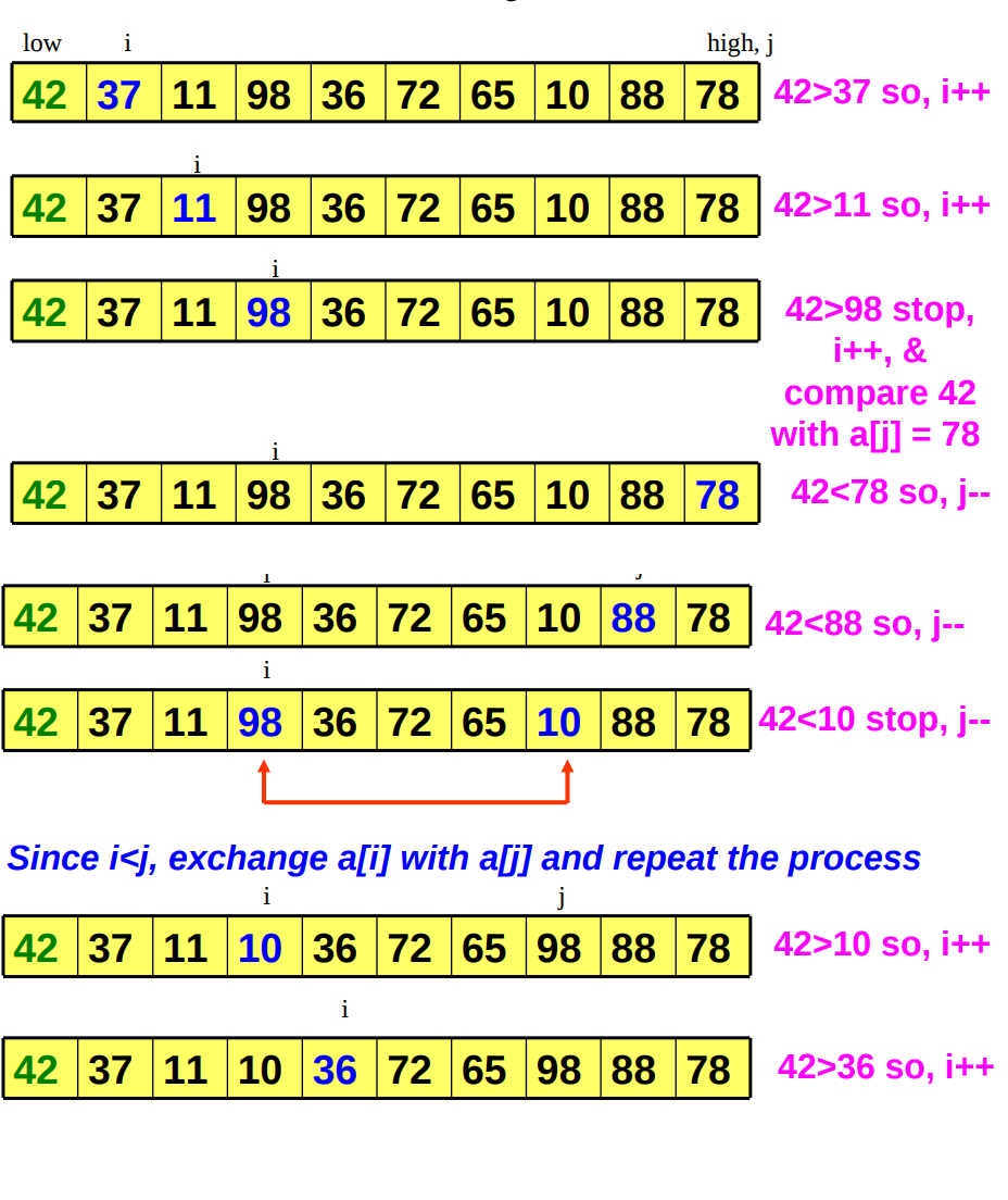
Let us assume an array A[10]={42,37,11,98,36,72,65,10,88,78}. We have to sort this array using quick sort.


// to swap two numbers
void swap(int* a, int* b)
{
    int t = *a;
    *a = *b;
    *b = t;
}

/* a[] is the array, p is starting index, that is 0, and r is the last index of array. */

void quicksort(int a[], int p, int r)
{
    if(p < r)
    {
        int q;
        q = partition(a, p, r);
        quicksort(a, p, q);
        quicksort(a, q+1, r);
    }
}

int partition (int a[], int low, int high)
{
    int pivot = arr[high]; // selecting highest element as pivot
    int i = (low - 1); // index of smaller element
    for (int j = low; j <= high- 1; j++)
    {
// If current element is smaller than or equal to pivot
        if (arr[j] <= pivot)
        {
            i++; // increment index of smaller element
            swap(&arr[i], &arr[j]);
        }
    }
    swap(&arr[i + 1], &arr[high]);
    return (i + 1);
}
Merge Sort
Merge sort is a comparison based sorting algorithm. It is based on divide and conquer rule. In this algorithm we divide the array into equal halves first and then combines them in a sorted manner. This sorting algorithm suffers from space complexity but is it a stable algorithm because it preserves the input order of equal elements in the sorted output.
It is most respected and trusted sorting algorithm because of its time complexity in worst-case being Ο(n log n).
Algorithm
Step 1: if it is only one element in the list it is already sorted, return.

Step 2: divide the list recursively into two halves until it can no more be divided.

Step 3: merge the smaller lists into new list in sorted order.
Merge sort keeps on dividing the list into equal halves until it can no more be divided. Then, merge sort combines the smaller sorted lists keeping the new list sorted too.
Example,
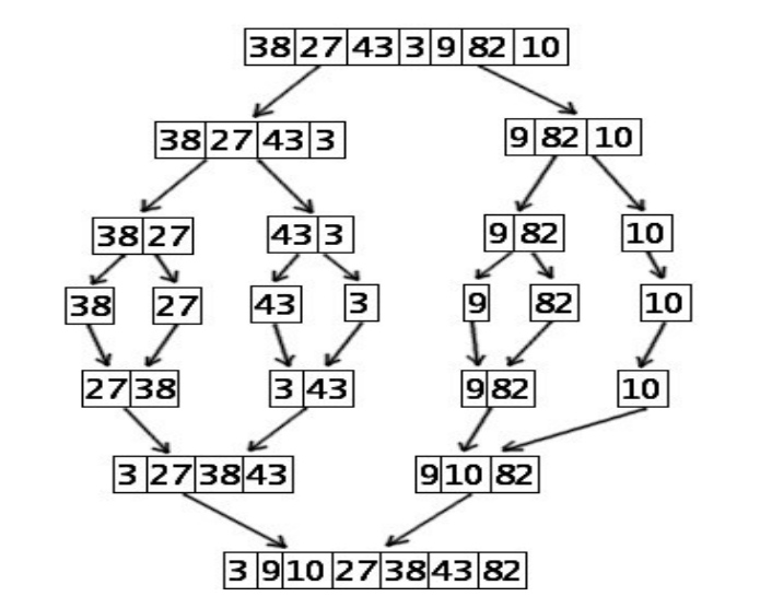
Let us take an example of an array A[7]={38,27,43,3,9,82,10}. We have to sort it using Merge sort.

void mergeSort(int a[], int p, int r)
{
    int q;
    if(p < r)
    {
        q = (p + r) / 2;
        mergeSort(a, p, q);
        mergeSort(a, q+1, r);
        merge(a, p, q, r);
    }
}

// function to merge the subarrays
void merge(int a[], int p, int q, int r)
{
    int b[5]; //same size of a[]
    int i, j, k;
    k = 0;
    i = p;
    j = q + 1;
    while(i <= q && j <= r)
    {
        if(a[i] < a[j])
        {
            b[k++] = a[i++]; // same as b[k]=a[i]; k++; i++;
        }
        else
        {
            b[k++] = a[j++];
        }
    }
    while(i <= q)
    {
        b[k++] = a[i++];
    }
    while(j <= r)
    {
        b[k++] = a[j++];
    }
    for(i=r; i >= p; i--)
    {
        a[i] = b[--k]; // copying back the sorted list to a[]
    }
}
Shell Sort
Shell sort is the generalization of insertion sort. It improves insertion sort by comparing elements separated by a gap of several positions. In this algorithm we avoid large shifts. This algorithm uses insertion sort on a widely spread elements, first to sort them and then sorts the less widely spaced elements. This spacing is termed as interval. We calculate the intervals using Knuth’s formula i.e., h=h*+1 where, h is interval with initial value 1.
Average and worst case complexity of this algorithm are Ο(n), where n is the number of items.
Algorithm
Step 1: Initialize the value of h

Step 2: Divide the list into smaller sub-list of equal interval h

Step 3: Sort these sub-lists using insertion sort

Step 4: Repeat until complete list is sorted
Example,
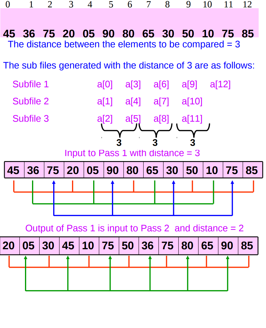
Let us take an example of an array A[13]={ 45,36,75,20,05,90,80,65,30,50,10,75,85}. We have to sort it using Shell sort.


This article contains basic idea of sorting and searching. It is a tutorial on sorting and searching techniques used in data structures and algorithms.
Was this article helpful? Must share your views in the comment section below.
Keep visiting our Tech Blogs and stay updated with our latest blog posts.

